Enforcing Contact Constraints Using Penalty Contact Method in Abaqus
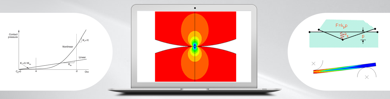
There are two primary methods through which normal direction contact constraints can be enforced in Abaqus/Standard: the traditional direct Lagrange multiplier method and a penalty-based method. The fundamental difference between the two methods is that the Lagrange multiplier method exactly enforces the contact constraint by adding degrees-of-freedom to the problem while the penalty method approximately enforces the contact constraint through the use of “springs” without adding degrees-of-freedom. The penalty method is depicted schematically in Figure 1. The lower surface is the main node and the upper surface is the secondary node. While the overclosure has been exaggerated, it is clear that the spring of stiffness kp resists the penetration of the secondary node into the main surface.
A large class of problems exists where the extra accuracy that is possible with the Lagrange multiplier method is not consistent with the approximations that are made (i.e., coarse meshes). Often times in these problems, adequately capturing load transfer through the contacting interface is more important than precise enforcement of the zero-penetration condition. The penalty method is attractive in such applications because it is usually possible to trade off some small amount of penetration for improved convergence rates.
The penalty method implementation in Abaqus attempts to choose a reasonable penalty stiffness based on the underlying element stiffness. If the default penalty stiffness is not suitable, options to scale the penalty stiffness are available. It is also possible to prescribe the penalty stiffness directly. If the scaled or user-prescribed penalty stiffness becomes very large, Abaqus automatically invokes special logic that minimizes the possibility of ill-conditioning. Advantages and disadvantages of each method are listed in Table 1.
| Table 1: Direct Lagrange multiplier vs. penalty method | |||
| Direct Lagrange multiplier contact | Penalty contact | ||
| Advantages | Disadvantages | Advantages | Disadvantages |
|
· Exact constraint enforcement (zero penetration) · Easy to recover contact forces ·No need to define contact stiffness |
· Larger system of equations · Difficult to treat over constraints · Sensitive to chattering |
· Number of equations does not increase · Easier to treat over constraints |
· Approximate constraint enforcement (finite amount of penetration) · Difficult to choose proper penalty stiffness |
Linear and Non-linear Penalty Stiffness
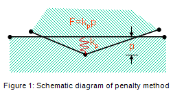
With the non-linear penalty stiffness approach, the penalty stiffness has constant initial and final values; these values serve as bounds for an intermediate overclosure regime in which the stiffness varies quadratically. A schematic comparison of the pressure-overclosure relationships for the linear and nonlinear penalty methods is given in Figure 2:
The various parameters used for defining the non-linear pressure-overclosure relationship are given below:
- Klin– Linear stiffness used for linear penalty contact. The default value is 10 times a representative underlying element stiffness.
- C0– Clearance at which contact pressure is zero. The default value is zero.
- Ki– Initial stiffness. The default value is 1/10 of the linear penalty stiffness.
- Kf– Final stiffness. The default value is 10 times the linear penalty stiffness.
- d – Upper quadratic limit. The default value is 3% of the characteristic length computed by Abaqus/Standard to represent a typical facet size.
- e – Lower quadratic limit. The default value is 1% of the characteristic length computed by Abaqus/Standard to represent a typical facet size.
- er= e/d – Lower quadratic limit ratio. From the default values of parameters d and e, the default value for er is 0.3333.
The default values for these parameters are based on the characteristics of the underlying elements of the secondary surface. For two elements with dissimilar materials in contact with each other, the contact penalty stiffness value chosen will be based on the material stiffness of the softer material. User control for changing the default values is provided. The nonlinear penalty method has the following characteristics:
- A relatively low penalty stiffness is used while the contact pressure is small. This serves to reduce the severity of the discontinuity in contact stiffness when the contact status changes.
- The smooth increase of the penalty stiffness with overclosure helps avoid inaccuracies associated with significant penetrations without introducing additional discontinuities.
The low initial penalty stiffness typically results in better convergence for problems that are prone to chattering with linear penalty contact, and the higher final stiffness keeps the overclosure at an acceptable level for problems with high contact pressure. Nonlinear penalty contact tends to reduce the number of severe discontinuity iterations due to a smaller initial stiffness; however, it may increase the number of equilibrium iterations due to the nonlinear pressure-overclosure behaviour. Hence, it cannot be guaranteed that nonlinear penalty contact will result in a reduction of the total iteration count compared to linear penalty contact.
As discussed above, Abaqus attempts to choose reasonable penalty stiffness values based on the underlying element stiffness. Experience has shown that for stiff or blocky problems the default penalty stiffnesses chosen by Abaqus produce results that are comparable in accuracy to results produced using the direct Lagrange multiplier method but usually at less expense in terms of memory and CPU time. Experience has also shown that for bending-dominated problems the default linear penalty stiffness can often be scaled back without any significant loss of accuracy. Furthermore, scaling back the penalty stiffness for bending-dominated problems has been seen to sometimes dramatically increase the convergence rate. These experiences are demonstrated by the following examples.
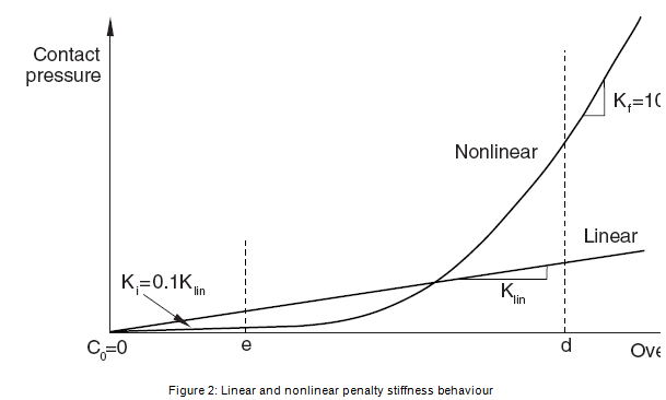
Example: Hertz contact
This example consists of two elastic cylinders in contact as depicted in Figure 3. The node-to-surface formulation with matching meshes was used. Cases were run using the direct Lagrange multiplier method, the linear penalty method with default stiffness, and the linear penalty method with default stiffness scaled back by two orders of magnitude. Results from the three cases are presented below in Table 2.
As expected, the direct Lagrange multiplier case produces zero penetration while the cases that use the penalty method produce finite penetrations. In this example, scaling down the penalty stiffness by a factor of 100 results in a 55x increase in the penetration. It can be seen that for this example the default penalty stiffness predicts a peak stress that differs by only 1.5% from the peak stress that is computed using the direct Lagrange multiplier method. If the penalty stiffness is scaled back by a factor of 100 then the predicted peak stress decreases considerably and differs by 47% from the peak stress that is computed using the direct Lagrange multiplier method. The significant decrease in peak stress is due to the combination of displacement controlled loading and the compliance at the contact interface with the penalty method.
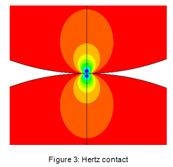
Table 2: Hertz contact results
| Penetration | Peak Stress | |
| Direct Lagrange | 0 | 1.201E5 |
| Linear Penalty, default stiffness | 4.482E-6 | 1.183E5 |
| Scaled Linear Penalty, Sf = 0.01: | 2.492E-4 | 6.334E4 |
Example: Bending-dominated contact
This example consists of a three-point bending test of an elastic-plastic beam as depicted in Figure 4. The node-to-surface formulation and half symmetry have been used. Cases were run using the direct Lagrange multiplier method, the linear penalty method with default stiffness, and the linear penalty method with default stiffness scaled back by two orders of magnitude. Results from the three cases are presented below in Table 3.
As expected, the direct Lagrange multiplier case again produces zero penetration while the cases that use the penalty method produce finite penetrations. In this example however, it can be seen that both cases that use the penalty method predict a peak stress that is practically identical to the peak stress computed using the direct Lagrange multiplier method. The behaviour that is seen in this example where a relatively small penalty stiffness produces quite accurate stress results generalizes to a very large class of bending-dominated problems. It can also be seen that in this example the penalty method produces a more economical solution as measured by iteration counts that decrease as much as 14%.
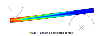
Table 3: Bending dominated contact results
| Penetration | Stress | Iterations | |
| Direct Lagrange | 0 | 2.416E4 | 130 |
| Linear Penalty, default stiffness | 1.004E-7 | 2.416E4 | 117 |
| Scaled Linear Penalty, Sf = 0.01 | 1.015E-5 | 2.416E4 | 112 |
Usage
The penalty method is applicable to all contact formulations. The linear penalty method is used by default for the finite sliding surface-to-surface formulation (including general contact) and for three-dimensional self-contact; the direct Lagrange multiplier method remains the default constraint enforcement method in some cases. In order to activate the penalty method use the options listed below.
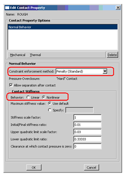
Abaqus/CAE
In the Interaction module, open the Interaction Property Manager by selecting Interaction → Property → Manager. Select the appropriate interaction and click Edit to receive the Edit Contact Property dialog. Select Mechanical → Normal Behaviour → constraint enforcement method: Penalty (Standard) → behaviour: [Linear | Nonlinear] as shown below:
Input file
The penalty method is selected with the following keyword options:
*SURFACE BEHAVIOR, PENALTY = [ LINEAR | NONLINEAR ]
The data lines can be used to modify the default settings for either the linear or nonlinear approaches.
Mr Vignesh P has done his B. Tech in Mechanical Engineering from Guru Nanak Engineering College (Hyderabad) which is affiliated to JNTU, Hyderabad. He has done his Masters in Science in Automotive Engineering from M.S Ramaiah School of Advanced Studies (Bangalore) affiliated to Coventry University, United Kingdom. He has a total experience of 6.5 years in FEA domain. He has worked on software solutions like Abaqus, Ansys, and Hypermesh. He has handled projects like stent deployment simulations, seismic analysis of dams, optimization of industrial planetary gearbox, etc. He has been with EDS Technologies Pvt. Ltd. for more than 5 years helping customers to develop methodologies for their projects, supporting customers/users on their queries, trainings etc. of both academia (IITs, NITs) and commercial customers.